Estimating Continuous Probabilities

This is a much more difficult problem than the problem of discrete probability estimation. This is because, if $P(x)$ is a probability distribution on a continuous variable, $x$, we have to estimate its value at an infinite number of points $x$. Of course we will only have a finite sample of data points with which to do this. Clearly, some type of interpolation between these points will be required. There is a substantial literature on this problem, which is known as probability density estimation. See, for example, Chapter 2 of Neural Networks for Pattern Recognition by Bishop, or chapters 3 and 4 of Pattern Classification and Scene Analysis by Duda and Hart for a treatment.

This problem will be important to us because we will often have a continuously varying measurement which will be used to make a classification. Thus, we will be attempting to estimate $P(c\vert m)$, where $c$ is the classification and $m$ is the value of the measurement. That can be done by estimating $P(m\vert c)$, that is the probability distribution for the values of the measurements for each classification, which is related to $P(c\vert m)$ through Bayes rule. The estimation of $P(m\vert c)$ is one of density estimation.

Methods of density estimation fall into two classes: parametric and non-parametric. Parametric approaches assume a particular form for the probability distribution. There are some parameters which are adjusted to make the distribution most like the data. For example, a common approach for one-dimensional data is to assume that the data comes from a normal or Gaussian distribution. This distribution is specified with two parameters, the mean and the standard deviation. It turns out that the best way to set those parameters is use the mean and the standard deviation of the data. It can be shown that these are the maximum likelihood estimates. The problem with this approach is that the assumed form of the distribution might not be appropriate for the problem.

An example of a non-parametric method is a histogram. To make a histogram, you simply divide the region which contains the data into a number of equal sized sections or bins; the estimate of the density for each section is the fraction of the data which falls inside that bin. In other words, to estimate of $P(x)$ for any $x$, find the bin that $x$ is in, say that is the $i$th bin, and use the estimate $P\sim N_i/N$, where $N$ is the number of data points used to make the histogram, and $N_i$ is the number of data points in the $i$th bin.

The choice of the bin size determines how smooth the data appears. If the bin-size is very small, the density will appear very spikey; if the bin size is large, important features of the data might be washed out. One of the problems with histograms is that one never knows how to set the bin size. Another problem is that they can only be used on low dimensional data.

As an example of density estimation, consider the following set of numbers:

 37    28    36    42    26    27    37    48    26    19    48    42
 33    38    20    11    28    40    48    28    41    44    27    46
 17    28    14    44    21    48    29    35    32    14    20    43
 18    25    38    24    27    43    46    24

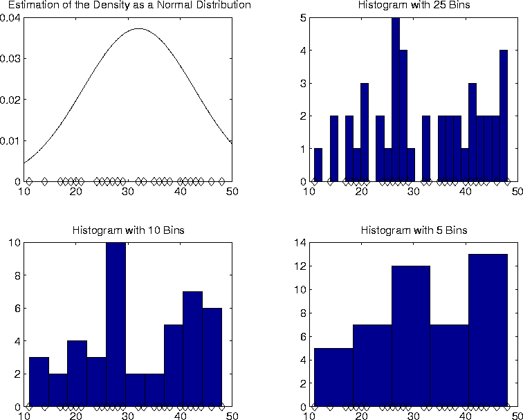
Suppose we want to model a probability distribution which may have produced the data. First, model the data as a normal distribution. The mean of the data is $m= 32.05$. The standard deviation of the data is $\sigma = 10.7$. Thus, the distribution could be modelled as a normal distribution with these values for the mean and standard deviation. This is shown as the first graph in figure  (the data is also shown as diamonds on the bottom of the graph).

To produce a histogram, divide the region which contains the data in to a number of bins. In this case the data lies in the interval $11$ to $48$. The remaining graphs in figure  show histograms for different bin sizes. Notice that the histograms seem to show that the distribution has two peaks. The Gaussian approximation, misses this, of course.

Figure: Examples of density estimation. The data is shown as diamonds at the bottom of the graphs. The first graph shows a Gaussian approximation to the distribution. The others show histograms with varying bin sizes.