B. The Gaussian or Normal Distribution

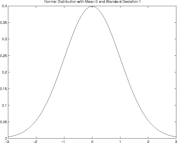
There is a very common and important example of a continuous probability distribution. This is the Gaussian, or Normal distribution, also called a bell-shaped curve. It looks like this figure .

Figure: A normal or Gaussian distribution with zero mean and unit standard deviation.

It is determined by two numbers, the location of the peak and the width. Mathematically, the two parameters which define it are the mean $m$ and the standard deviation $\sigma^2$. The mathematical form of the distribution is

$$P(x\vert m,\sigma^2) = \frac{1}{\sqrt{2 \pi}\sigma} \exp\left[-\frac{\left(x-m\right)^2}{2 \sigma^2}\right]$$

. The normal distribution is important because the sum of a set of independent variables drawn from almost any distribution approaches Gaussian as the number of variables goes to infinity. So, for examples, means tend to be Normally distributed. This result is called the central limit theorem.

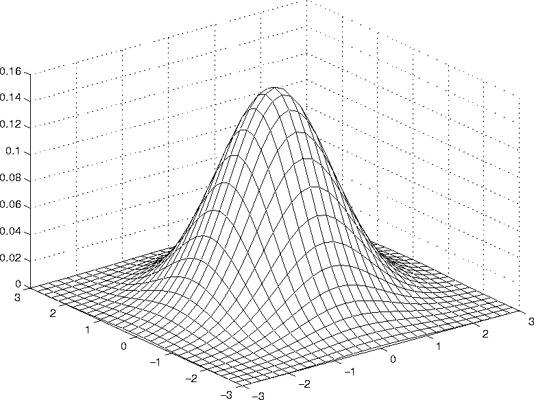
There is a multidimensional version of the Normal distribution. It is called a multi-variant Gaussian; it is shown in two-dimensions in figure .

Figure: A two-dimensional Gaussian

In this case it is defined by the centre of the peak, two directions of spread and two widths along those two special directions.