SpiNNaker Project: Applications - Other.
Multilayer Perceptrons
|
The PDP2 project is implementing an entirely different kind of neural network:
a non-spiking "classical" multilayer perceptron (MLP) model. By far the most
popular type of computational neural network, the MLP consists of a number
of neurons, (or "units") that compute some simple nonlinear threshold function
on the sum of their inputs. Like spiking networks, connections between units
are through synapses (or "weights") that are plastic and hence change weight
while the data passes through the network. MLP models, however, have
important differences. Typically weights are only plastic for a certain time, the
"training phase" and then are fixed during the "test phase". Each phase consists
of some number of examples, individual data items presented to the network.
This in turn implies that the MLP has no time model, or to be exact, a
discrete-time model. Contrasting strongly with spiking models: the MLP model
thus has a synchronous dataflow. In addition, the most popular learning
technique is backpropagation, a method that involves propagating errors from
output units backwards through the network to update the weights. Both of
these properties present challenges to the SpiNNaker architecture.
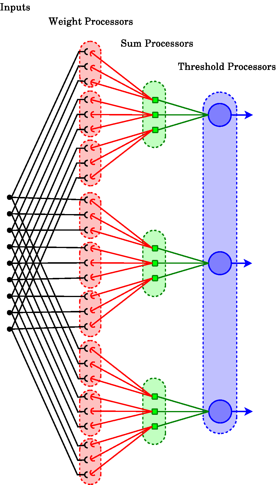
We have solved the synchronous dataflow problem using a new technique - "update-on-demand", that computes partial results and forwards them on through the network as soon as they are available. The backpropagation algorithm, which presents challenges for the source-routed SpiNNaker topology because it is effectively bidirectional, we solve using a matrix remapping method that distributes the processing between cores [X. Jin, M. Lujan, M. M. Khan, L. A. Plana, A. D. Rast, S. Welbourne, and S. B. Furber, "Efficient Parallel Implementation of a Multi-Layer Backpropagation Network on Torus-connected CMPs" in Proc. 2010 ACM Conf. Computing Frontiers (CF'10), 2010, pp. 89-90]. The SpiNNaker MLP implementation models networks using the Lens (http://tedlab.mit.edu/~dr/Lens) specification and will provide support for both feedforward and recurrent networks. Initial support is provided for networks defined at a Group level; future plans may include support for Unit-level definitions. Full support is provided for Group-to-Unit and Unit-to-Unit connectivity. A SpiNNaker package plugin for Lens allows Lens scripts to be implemented directly on SpiNNaker using the automated PACMAN path.SpiNNaker MLP mapping The figure to the right shows an MLP implementation on SpiNNaker. Each dotted oval is one processor. At each stage the unit sums the contributions from the previous stage. One processor may implement the input path for more than one final output neuron (shown here for the threshold stage). |
|
Heat Equation Solution
|
The Heat Equation is a partial differential equation that describes the variation in temperature over time in a region, given an initial temperature distribution and boundary conditions.
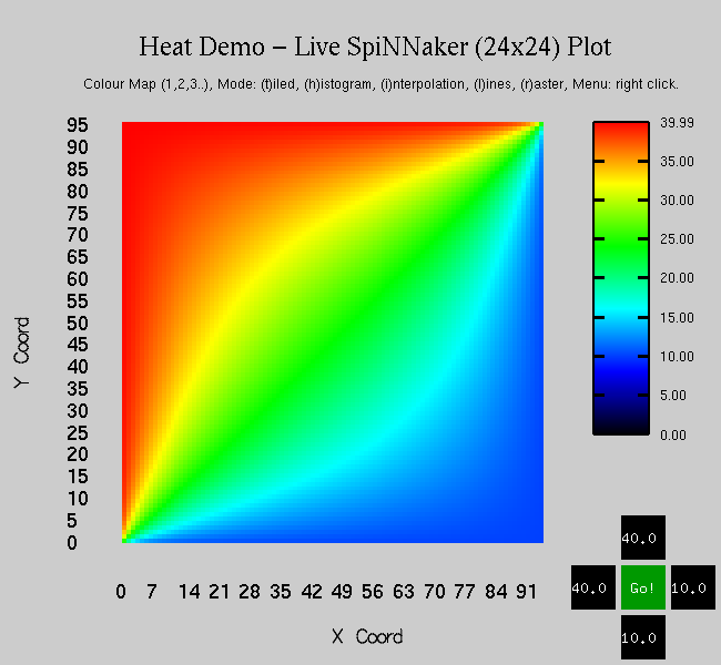
Relaxation methods are iterative numerical methods for solving systems of equations, including nonlinear systems. In particular, they are used to solve finite-difference discretizations of differential equations, such as the Heat Equation. These methods are well-suited for parallel implementations following a Single Program Multiple Data (SPMD) model: multiple autonomous cores simultaneously execute the same program with different data and use messages to communicate with each other. Using a relaxation method to solve the Heat Equation is easily and efficiently mapped to SpiNNaker. The entire region is partitioned into sub-arrays of points and distributed across the machine. In the extreme, every core is assigned a single point. Each core can then compute the corresponding temperatures and distribute them to its neighbours using SpiNNaker's efficient multicast communication infrastructure. The figure to the left shows a snapshot of the output of a Heat Equation Solver running on a SpiNNaker system. Each square represents the temperature at a given point in the region. The user can control the temperatures of the North, South, East and West boundaries and view the evolution of temperatures over time. The figure shows the North and West boundaries at 40 °C and the East and South boundaries at 10 °C. |